Solver

The solver solver runs the simulation, by advancing the solution in time. Thanks to the preparatory work done by preproc, the duties of solver, besides raw computing, are minimal. Before starting time integration, solver only needs to:

• read the cube-specific files, and assign cube data to each MPI rank;
• compute the pointers which will be used in the time advancement;
• define the time advancement routines;
• complete the setup of the MPI communications;
• load the restart field.

After this part is complete, the execution proper starts. The algorithm which integrates the IB into the discrete solution of the Navier-Stokes equations is being documented in a paper currently under development.

The main program

The file solver.cpl is the main program of the solver. It contains most of the operations which are independent from a specific flow type: input-output, BCs, MPI communications, runtime computing of some flow statistics and GPU initialization have their dedicated files io.cpl, bc.cpl, comm.cpl and gpuInit.cpl in the folder modules-solver/.

Pointers

solver computes the solution only at grid points laying in the fluid (internal points). For computational efficiency, arrays of pointers to the internal points are pre-computed and stored. Distinct arrays are used:

• time advancement pointers: they store addresses of the collocation points where at least one of the velocity components lies in the fluid region;
• pressure correction pointers: they store addresses of the collocation points where the pressure correction routine has to be performed; two arrays exist for the red-black ordering. The programming logic behind the identification of pressure correction points is complex, as pressure correction is not applied to internal points belonging to non-periodic BCs;
• BC pointers: they store addresses of the collocation points where BCs are applied; they are obtained from the boolean maps computed by preproc, and are also used to compute flow rates.

Pointers are highly advantageous from a computational viewpoint, but introduce additional complexity when working in heterogeneous memory environments (e.g. CPU-GPU). Pointers computed on CPUs cannot be used on GPUs, and viceversa (unless managed memory is used). On the other hand, computing pointers is a sequential operation, and becomes very slow on GPU. Although computing pointers is a one-time operation, a hybrid approach is implemented:

• the time advancements pointers, which are simple to define, are computed sequentially on GPU asynchronously;
• the pressure correction and BC pointers, which are more complex to define, are computed on CPU; the same holds for the interaction with complex data structures as the boolean maps. Pointers are then subtracted by an arbitrary base pointer inside the data structure to switch from addresses to byte shifts, and then copied to GPU. Once on GPU, the byte shifts are summed again to another base pointer, restoring their pointer nature. This last operation can be (and actually is) performed in parallel on GPU;
• synchronization is imposed.

Input-output operations

The file io.cpl contains the procedure which distributes cubes among ranks, as well as the routines responsible for the read-write operations of the different data structures. The file is also USEd by the postprocessing utility createVTK.cpl.

Loading cube files requires opening and closing them several times, to reduce file system load at a slight expense of execution times; data consistency is checked at every step. The loading procedure is as follows:

• the shared datafile general-info.dat is read by all the MPI ranks (an error is triggered whenever the number of ranks exceeds nTotCubes);
• the array of cube IDs is subdivided randomly among the available ranks, such that each rank has (approximately) the same number of cubes;
• cube locality (i.e. which rank loads which cube) is established, and the information is shared among ranks, to allow writing the connectivity information needed for the MPI communications (an error is triggered whenever locality is not correct);
• the connectivity of each cube (i.e. for each cube, the rank of each neighboring cube) is established;
• the number of points contained in each cube is read (an error is triggered whenever cubes have different number of points);
• the IB coefficients and boolean maps for non-periodic BCs for each cube are loaded.

The random distribution of cubes among ranks already provides a relatively balanced load. For a proper (static) load balancing, the only step left is the solution of a graph partitioning problem, as done for example by Jansson et al. (2019). Once the graph is partitioned, by assigning the cube ID to each rank, the rest of the uploading procedure remains unchanged, and no moving of heavy data structures (such as the IB coefficients) is needed between ranks.

Communications

The program accepts domains decomposition in all three spatial directions, therefore, up to 26 communications may be performed by each cube (6 faces + 12 edges + 8 vertices). More than one cube can be assigned to each rank. Since multiple same-length buffers may happen to be exchanged by two ranks at the same time and in the same direction, buffers must be discriminated with MPI tags. Communications are uniquely identified by the ID of the sending cube and the direction in which the communication takes place (for example, from the sending cube to the receiving cube in the x direction). Unique tags are computed for each communication as:

$tag = (sndCubeID-1) \times 26 + commNum -1$

where commNum is an integer associated to a communication in a specific direction, from the sending cube (see table below):

Faces	Direction
1	Xprev
2	Xnext
3	Yprev
4	Ynext
5	Zprev
6	Znext

Edges	Direction
7	XnextYnext
8	XprevYnext
9	XnextYprev
10	XprevYprev
11	YnextZnext
12	YprevZnext
13	YnextZprev
14	YprevZprev
15	XnextZnext
16	XnextZnext
17	XnextZprev
18	XprevZprev

Vertices	Direction
19	XnextYnextZprev
20	XprevYnextZprev
21	XnextYprevZprev
22	XprevYprevZprev
23	XnextYnextZnext
24	XprevYnextZnext
25	XnextYprevZnext
26	XprevYprevZnext

Therefore, for the connectivity between ranks to be fully established, for each communication direction and cube the following information must be known:

• ID of the receiving cube where the buffer is sent;
• MPI rank where the receiving cube is loaded;
• MPI tag for the sending buffer;
• MPI tag for the receiving buffer.

The MPI communications are currently implemented with a procedure that involves three copy steps:

1. data for a given communication are copied to the corresponding sending buffer;
2. the MPI_Isend/MPI_Irecv call is posted, and the program then waits until all the ranks are synchronized before continuing;
3. data are copied from the receive buffer to the main data structure.

In alternative, a shortcut for communications between cubes belonging to the same rank is available. The shortcut not only saves one copy in the procedure, with better performance and less MPI overhead, but is also needed due to the dual CPU-GPU nature of the program. Indeed, GPU-aware MPI allows direct GPU-GPU copies between addresses belonging to different devices, but not between addresses of the same device: MPI_Send/MPI_Recv calls must be avoided in this case. Finally, it is important to mention that the program assumes the use of GPU-aware MPI to work with multiple GPUs.

The currently implemented MPI communications are not optimized yet. Some steps (in order of increasing complexity) towards increased efficiency are:

• for GPU, enable the asynchronous execution of kernels used to copy data from the data structure to the send/receive buffers;
• post the MPI_Irecv call before the routine after which the corresponding MPI_Isend call is, to overlap computations and communications;
• write a second communications routine to execute red-black communications for the pressure iterative solver which contains most of the communications performed in the timestep;
• skip the usage of sending buffer by using MPI_Datatype arrays (becomes a two-copies procedure for both in-rank and out-of-rank communications);
• pack buffers of different cubes which are exchanged between two ranks to avoid excessive communication startup overhead;
• use MPI topology, together with static load balancing, to optimize the distribution of cubes between ranks in the same node;
• use one-sided operations such as MPI_Put/Get and MPI_Win_allocate` to skip rank synchronization overhead (this solution has been implemented but currently it does not work on GPU for MPI implementation which rely on UCX for network communications).

Boundary conditions

Implementing a new BC is a straightforward process. One should only pay attention to the dependence upon the (signed) direction of the normal of the boundary. A new BC should be added within the CASE structure used for routines inletBC and outletBC in the file modules-solver/bc.cpl.

Currently, only BC taking one value for pressure, velocity components of flow rate are supported. Whether the value is used for a Neumann- or a Dirichlet-type BC or not used at all (e.g. for an implicit zero-gradient BC as in outlet BC), it is up to the user.

The list of boundary conditions can be easily extended in the case of 1-point stencils. Less trivial is the extension to larger stencils, as the domain decomposition exposes the risk of segmentation fault if the BC's surface falls in an unlucky spot. In this last case, there is no other option except changing the domain decomposition. At the moment no check is implemented, so beware of segmentation faults.

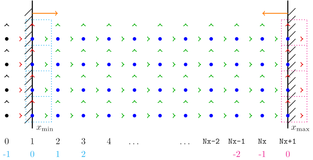
Except for no-slip BC, enforced through the IB coefficients, all the BC are imposed on planar surfaces. The BC planes are aligned with pressure points in the staggered grid. When the coordinate of a BC plane falls in-between two pressure grid points, it is applied to the nearest one.

Coordinates of points where BC is to be applied are saved in arrays of CPL pointers into the main data structure. These pointers are centered on the indices of the data structure which store the collocation points of the pressure on the surface where the BC is applied.

The figure below shows that, owing to the staggered grid, the implementation of BC changes when applied on different components of the velocity and on surfaces with different normal sign and direction.

Figure: example of explicit BCs applied at x=x_min and x=x_max. Green arrows are velocity points where equations are advanced in time, blue dots are pressure points where the pressure is corrected. Red arrows represent ghost velocity points where the BC is imposed. Black arrows and dots represent points not involved in the computations. Orange arrows indicate the boundary (signed) normal. Dotted squares represent grid points stored in the pointers arrays (cyan for positive normal, magenta for negative one). Colored numbers represent the relative index of the grid points with respect to the plane where the corresponding BC is applied.

Data structures and memory requirements

solver manages multiple cubes, therefore each cube needs private data. These data are stored in arrays with nCubes elements of the data structure needed by each cube.

The main data structures are listed and briefly commented below. The outer dimension nCubes of the arrays is omitted. Dimensions are reported from the outer one to the inner ones.

Cube metadata

Variable	Size	Description
rankCubesIdx	sizeof(int)	Stores the IDs of cubes loaded by the MPI rank.
cubeInfo	14 x sizeof(int) + 6 x sizeof(double)	Stores general data of the cube: • Cube ID • Number of fluid points • Grid spacing (for uniform grids) • Position of the first ghost point (p(0,0,0)) • Number of points in the cube • Global index of the first point (1,1,1) • Indices of last fluid points • Cube position in global grid
cubeConnectivity	4 x 26 x sizeof(int)	Stores connectivity data for cube-to-cube communication: • Neighboring cube IDs • Loading rank of neighbors • MPI send tags • MPI receive tags

Timestep

Variable	Size	Description
mainVariables	7 x (Nx+2)x(Ny+2)x(Nz+2) x sizeof(double)	Stores the seven main variables: p, u, v, w, uimbc, vimbc, wimbc at each grid point.
fldPtCount	sizeof(int)	Stores the total number of cube points with at least one fluid collocation point (used in time advancement).
temporaryVariables	6 x MAX(fldPtCount) x sizeof(double)	Stores support variables: utmp, vtmp, wtmp, newu, newv, neww needed for time advancement.
fldPtIndex	MAX(fldPtCount) x sizeof(double*)	Stores pointers into mainVariables for points with at least one fluid collocation point.
rbPtCount	2 x sizeof(int)	Stores the number of red and black cube points where pressure correction is applied.
rbPtIndex	2 x MAX(rbPtCount) x sizeof(double*)	Stores pointers into mainVariables where pressure correction is applied.

Boundary Conditions

Variable	Size	Description
cubeBCsNumber	sizeof(int)	Stores the number of boundary conditions (BCs) applied within the cube, excluding non-periodic and no-slip BCs.
cubeBCinfo	MAX(cubeBCsNumber) x 4 x sizeof(int)	Stores general information about each BC: • BC ID • Index of the plane where the BC is applied • Number of points where the BC is applied inside the cube • Signed normal of the plane
cubesBCsMaps	MAX(cubeBCsNumber) x sizeof(double*)	Stores pointers to boolean arrays. For a BC with normal x, the pointer references an array of size (Ny+2) x (Nz+2): • Y indicates the BC is applied at that point • N otherwise • The total number of Y is also stored in cubeBCinfo

Grid

Variable	Size	Description
xCoords	(Nx+2) x sizeof(double)	Stores the coordinates of the cube’s velocity collocation points in the x direction. Similar arrays: yCoords, zCoords for y and z directions.
xDiffs	(Nx+2) x 6 x sizeof(double)	Stores first and second derivative coefficients in the x direction. Similar arrays: yDiffs, zDiffs for y and z directions.

Statistics

Variable	Size	Description
statsArray	nStats x Nx x Ny x Nz x sizeof(double)	stores the cube statistics.