Preprocessor

In AMPHIBIOUS, preproc is the preprocessor responsible for splitting the computational domain (described either analytically or through STL files, which are preliminarily checked for quality) into cubes, and for elaborating the geometrical data needed by solver. This code has a modular organization, so that multiple configurations can be dealt with. Case-specific routines can be added for customization. Parallel execution is supported on CPUs only.

In the case directory, preproc writes preproc-log.dat, which contains useful information on the various stages of pre-processing, some warnings when the number of points is modified to make it even, and important information that is needed later, as the values of nDecompCubes and nTotCubes. Additional information is contained in the shared file general-info.dat.

preproc.cpl manages the following operations:

• bounding box (BB) and decomposition in cubes;
• mesh generation;
• geometry definition (STL or analytics);
• boundary conditions (BC);
• IB coefficients and geometrical features of the BC;
• IB coefficients for BC with wall-normal derivatives (optional)
• pruning empty cubes and writing data to memory.

Bounding box and cubes

The grid discretizes the region of space contained in the bounding box. The BB is a cuboid defined by its lower and upper boundary in the three directions; the coordinates of the BB boundaries are stored in the arrays bbMin and bbMax.

For analytically-described geometries, instead, it is up to the user to define the computational domain and its BB.

For STL geometries, preproc automatically retrieves the boundaries of the BB by scanning all the triangles contained in the STL files, to identify minima and maxima of the coordinates across all triangles, stored in bbMin and bbMax. In a second step, and only for the non-periodic directions, the BB is slightly shifted to avoid limit cases where a triangle happens to have one vertex exactly on the BB: this would cause finite-precision issues in the ray-casting step afterwards. Each non-periodic planar BB face, where the grid starts from, is thus shifted by $8 \times \epsilon$ outwards towards the solid; $\epsilon$ is the machine epsilon of float variables (since the STL triangles are by definition saved in single precision).

preproc is constrained to build cubes containing the same number of grid points. Therefore, cubes partially outside the bounding box may be generated. Their outer points are considered as solid points: their IB coefficients are computed accordingly, and they are ignored in the calculations performed by solver.

Mesh generation

XXX MISSING: SKETCH OF A CUBE/MESH XXX

The IBM adopts a staggered grid, with pressure defined at the center of a cubic cell and velocities defined at its faces. The code supports both uniform and non-uniform rectilinear grids, with arbitrary (one-dimensional) variations of the grid step size in every direction. The choice between uniform and non-uniform grid is made at compile time, by setting/unsetting the corresponding macro GRID_IS_NONUNIFORM in the file headers.cpl.

The process of mesh generation in the $x$ direction is described here with some detail (see the figure below for a sketch); the same goes for the other directions. The program generates Nx collocation points for the u velocity component; they fall within the interval [bbMin(0), bbMax(0)] defined by the extrema of the BB in the $x$ direction. TheseNx points are where the discrete Navier--Stokes equations might be solved; whether or not in a specific point this actually takes place (because the point is internal, i.e. in the fluid) depends on the geometrical complexity of the domain. For a simple channel flow, for example, all points inside the bounding box are internal points, since the bounding box and the computational domain coincide.

Example of uniform grid in the \( x \) direction with Nx=10. Blue dots represent pressure collocation points (automatically defined by preproc). Green arrows are the u velocity collocation points assigned by the user. Red arrows are the ghost nodes (automatically defined by preproc).

Ghost nodes are required to compute $x$ derivatives in the two extreme points at i=1 and i=Nx. The ghost nodes, at i=0 and i=Nx+1, are positioned outside the BB: in this way, pressure collocation points, automatically placed by preproc half-way between two velocity collocation points, end up exactly on the side of the BB. Therefore, given bbMin(0), bbMax(0) and the internal velocity collocation points x(1), x(2), ... x(Nx) computed in grids.cpl according to the specific grid distribution strategy, preproc computes the ghost points such that:

${ \left\lbrace \begin{aligned} &x^u_0 = x_{min} - 0.5 (x^u_1 - x_{min}) \\ &x^u_{Nx+1} = x_{max} + 0.5 (x_{max} - x^u_{Nx}) \\ &x^p_i = \frac{x^u_{i-1} + x^u_i}{2} \qquad \text{for $i=1:N_x+1$} \\ &x^p_0 = x^p_1 - (x^u_1 - x^u_0) \end{aligned} \right.}$

The obvious consequence is that the first and last points must be inside the BB for the grid to be valid, i.e.:

$x^u_1 > x_{min}, \quad x^u_{Nx} < x_{max} .$

This requirement is not checked, and must be fulfilled when creating a new grid type.

Also, the iterative algorithm used to enforce incompressibility implies a further restriction when periodic boundary conditions are used. Along periodic directions, the number of points given as input by the user must be even. Therefore, if an odd number is given, preproc automatically adds one point to make it even, and issues a warning in preproc-log.dat.

Non-uniform grids

The type of grid step variation is selected, independently for each direction, in the section NONUNIFORM_GRID of the settings.in file, by assigning the variables xGridType, yGridType and zGridType. The available mesh types can be found in modules-preproc/grids.cpl. Uniform (type u), hyperbolic tangent (type h) and cosine-spaced (type c) grids are implemented. The framework is such that new grid types can be easily added: one simply writes in grids.cpl the line of code for the desired variation of the grid step.

When using a non-uniform grid along periodic directions with STL geometry, additional requirements exist. They are addressed later.

Geometry

STL mode

This is by default how geometric information is provided to the code. Setting up preproc in STL mode requires to provide a list of STL files describing the input geometry. The surfaces delimiting the computational domain can be wall surfaces, periodic planes and surfaces where other BC are applied. The names of the STL files are listed in, and read from the input file settings.in. All the STL-specific actions are defined through functions contained in modules-preproc/geometry-stl.cpl.

The set of STL files must satisfy the following constraints:

• the computational domain (i.e. the fluid region) must be fully enclosed by the surface defined by the set of STL files;
• the normals of the triangles of the STL files must point towards the fluid domain;
• apart from those STL files where the wall-type BC w is used, the STL files must describe a planar surface, orthogonal to one of the coordinate axes. preproc checks planarity of these surfaces, and returns an error if the check fails (within a tolerance that depends on the grid spacing);
• periodic BC are applied to whole planar faces of the BB; fluid regions extending beyond a periodic plane will simply not be considered as fluid regions, and the behavior of preproc is in this case undefined;
• STL files for which periodic conditions are selected must be a pair: one STL for the lower boundary, and one for the upper boundary;
• the $y$ direction cannot be periodic, unless the calculation is tri-periodic, as for homogeneous isotropic turbulence;
• for an indefinite wall delimited by periodic planes, the IB coefficients near the boundary are computed assuming that the wall is symmetric with respect to the periodic plane. When using grid refinement in periodic directions, this condition is particularly strict as it requires the grid to be symmetric near the boundary of the domain. Referring to the grid figure above, this implies:

${\left \lbrace \begin{aligned} &x^u_1 - x_{min} = x_{max} - x^u_{Nx} \\ &x^u_2 - x_{min} = x_{max} - x^u_{Nx-1} \end{aligned} \right.}$

• the surface described by one STL file can take only one BC; to be described by the same STL file, two distinct surfaces must have the same orientation (and the same normal) with respect to the fluid domain, the same type of BC, and the same boundary value imposed at the boundary;
• multiple wall files are allowed; they are treated as one.

A set of STL files satisfying these constraints is processed correctly by preproc and solver. Not all constraints are (and some cannot be) checked at run time.

Analytic mode

To have preproc work in this mode, the macro GEOMETRY_IS_ANALYTIC must be defined before compilation.

All the analytic-geometry actions are defined through functions contained in modules-preproc/geometry-analytic.cpl. For generality, functions are defined as <function name><Geometry> in a geometry-specific file placed in the geometry-analytic directory; they are then linked to the global function it refers to via the line <function name>==<function name><Geometry>. This ensures that only the geometry-specific function has to be specified, while the modules-preproc/geometry-analytic module remains unchanged.

Setting up preproc in analytic mode requires four steps:

1. Fill in the section ANALYTIC_GEOMETRY of settings.in, by providing the dimensions of the bounding box (Lx, Ly, Lz), the number of computational boundaries (nFaces), and a list of nFaces types of boundary conditions, eventually completed by specific parameters.
2. Define the number of planes in which BC other than w and p are applied. This is done by the subroutine computenOtherBCFiles<Geometry>. An example is computenOtherBCFilesChannel in modules-common/specifics-channel.cpl.
3. Define the boolean function inBody<geometry>(x,y,z), which contains the analytical description of the geometry, and returns YES only if the point of coordinates (x,y,z) belongs to the solid. An example can be found in the modules-common/specifics-channel.cpl module, where inBodyChannel is defined.
4. Define the buildBoundingSquare<Geometry> subroutine. This is actually enabled twice for each non-periodic and non-wall direction only (once for the lower and once for the upper boundary). For each boundary, it fills the structure BSquareDelimiter by specifying the edges of the plane containing the boundary condition prescribed in the three Cartesian directions, and the direction of the wall-normal vector. An example for the plane channel flow is available in modules-common/specifics-channel.cpl: in this case the boundaries of the computational domain coincide with those where the boundary conditions have to be applied; however, other flows, like the flow around a solid body, can be studied with this infrastructure.

Once these functions are defined, preproc looks for cubes intersected by the boundary conditions chosen, flags every relevant point, and stores this information in the cube-specific file.

Boundary conditions

Different types of BCs are dealt with differently:

• wall BC (type w) is imposed via the IB coefficients, for what concerns velocity and Dirichlet-type for temperature;
• periodic BC (type p) are hard-coded in the communications between cubes (this is why periodic BC must be applied on whole faces of the BB);
• the other types are dealt with in two steps; preproc only manages their geometrical description, that is read later by solver, which links it to the corresponding BC type and executes the corresponding routine.

The boundary conditions are elaborated by preproc to identify the ghost points (GP), i.e. solid grid points for which at least one of the neighbors lies in the fluid, extracting the geometrical information needed by solver.

preproc checks first if periodic BC are present, and makes sure that all the non-wall STL files meet the requirement of being planar and orthogonal to one coordinate axis. Then, for each cube, preproc fills a list with the pressure external grid points nearest to the BC plane, and the boolean otherBCsPointsMap is set to YES to restrict them to points involved in the BC. The corresponding velocity points are also flagged. The lists and their length are eventually saved by preproc in each cube-specific file. This information enables solver to apply the BC only at the flagged points. Besides identifying points where BC will be applied, the STL files also define the interface between the computational domain and the external (solid) volume.

As described below, a competing ray-casting algorithm is used to discriminate internal (fluid) and external (solid) regions. The ray-casting is used for each grid point, considering as a whole the surface provided with STL files. Note that there are no explict checks on the STL quality, including watertighness in its intuitive sense: users can ran preproc for any ensemble of surfaces, the responsability to check whether the geometry simulated is the intended one rests on them.

IB coefficients

The IB coefficients are computed as the sum of all the 6 contributions from the stencil of the 3D Laplacian operator, assembled in the subroutine starSTL in the temporary variable pointStar.

At the higher level, calcImbCoeffs, which is called once for each the (staggered) velocity grids, performs the following actions:

• it initializes the boolean mask isPointInside;
• it calls markInsidePts, which fills isPointInside and sets to SOLID of all external points;
• it calls starSTL, which computes the IB coefficients;
• it calls inPlaneBCcoeffs and imbBCcoeffs, which set the IB coefficients of points where BC other than p and w (periodic and wall) are imposed.

Ray-casting and IB coefficients for solid walls

The identification of internal points and the evaluation of IB coefficients are two distinct steps.

Internal points are identified via a ray-casting algorithm in find-inside.cpl and invoked through the subroutines markInsidePts and checkIfSolid. The algorithm for each grid point uses first 3 rays directed in random directions; when the 3 attempts lead to a non-unanimous vote, 8 additional random rays are used. The intersection between ray and triangle is evaluated using the ray-perturbation method to deal with degenerate cases.
The information on which point is internal or external is stored in the boolean mask isPointInside.

The evaluation of the IB coefficients is contained within the starSTL subroutine. For each STL triangle belonging to a wall, all grid points are checked. The variable pointStar, which is an array of size $3 \times 2$, stores the distance from the single grid point from to wall triangle. The first index of this variable signals which direction is being considered, and the last index stores the sign of the distance from the nearest wall. The relative distance is computed with the function intersect. The triangle is projected over the plane perpendicular to each Cartesian axis, the baricentric coordinates are computed to establish whether the grid point falls within the projected triangle; when it does, the (signed) distance from the grid point to the triangle along the considered direction is computed. If this distance is lower than the distance between grid points, it is saved in pointStar, and then added to the IB coefficient.

IB coefficients for wall-normal derivative

Wall-normal derivatives are discretized with a finite-difference scheme using a stencil with 3 non-equally-spaced points. Quadratic interpolation is used to achieve second-order accuracy. The already flagged ghost points (GP) are used. However, additional coefficients are needed.

Wall-normal derivatives (may) appear in the boundary condition for the passive scalar equation, and require the macro USE_HT to be defined. However, the approach is general: wall-normal derivatives can be used in the BC of other equations, by adding a single line to preproc (and by coding the additional BC in solver).

Coefficients and some extra data are stored in the structure neumannData, that gets saved in .bin files with the same name. The structure is computed and stored only when preproc is compiled with the macro WALLT_IS_NEUMANN. Whether neumannData will be then actually read and used by solver depends on the BC prescribed in settings.in

Using wall-normal derivatives requires two steps.

Step 1: distance from the boundary

Three algorithms are available to find the direction used to compute the distance between each GP and the boundary. They are used in increasing order of robustness (and decreasing order of accuracy), until one succeeds. When an algorithm provides multiple values, the shortest distance is selected. This strategy is inspired by the work of Mittal et al (2008).

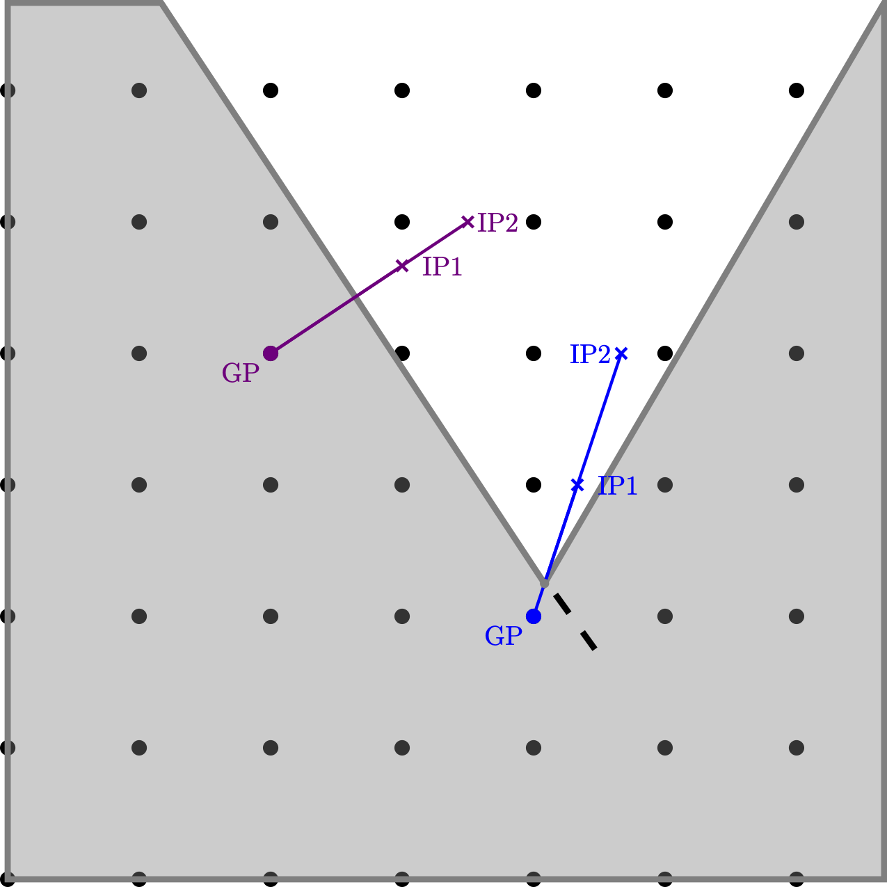
1. The distance is computed along the line made by the normal to a neighbouring STL triangle. In most cases, this line intersects the triangle and therefore solves the problem (purple GP in the figure below)
2. The distance is computed as the minimum distance between the GP and each point on the edge of the STL triangle (blue GP in the figure below)
3. The distance is computed along the Cartesian direction. This is equivalent to a staircase description of the domain

The last (worst) option becomes necessary only in rare cases, where geometric singularities (e.g. sharp cuspids) are accompanied by poor grid resolution.

The search for the normal starts with the STL triangles within $2\Delta x$ of the point, and explores all triangles in expanding concentric circles around the point. The search stops at a radius of $10 \Delta x$, when a warning is issued about poor grid quality. Aside from insufficient resolution, troubles may be expected with strongly anisotropic grid spacing near complex geometries.

Once a straight line to compute the distance is available, two image points (IP) are positioned on it. They belong to a grid plane, i.e. they share at least one coordinate with the grid. IP1 coincides with one of the grid points surrounding the GP, while IP2 is on the next plane found by prolonging the segment GP-IP1 (the distance between IP1 and IP2 must be larger than a threshold to avoid numerical problems).

Ghost and image points: a 2D sketch. The shaded area is the solid body, with the overlapping grid. Two GP types are shown, together with their pair of IP, illustrating cases where different strategies are necessary: strategy (1) for the purple GP, and strategy (2) for the blue GP. Note how the line defining the distance is not necessarily normal to the boundary.

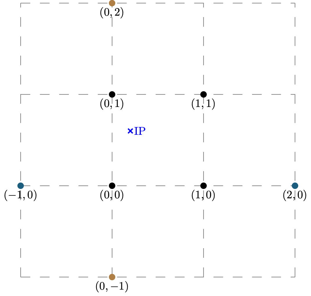
For each IP, a planar interpolation stencil made up of 6 in-plane neighbors is defined, as shown in the example below. By default the points at 0,1,2 are considered, in each direction. Whenever the point 2 is not available because is outside the cube boundary, the stencil is modified to include -1,0,1.

Interpolation stencil. Each IP has 4 surrounding interpolation points (in black), plus 1 blue and 1 orange point, either forward or backward depending on whether the forward point belongs to the cube.

Step 2: interpolation coefficients

Once the interpolation stencil is known, the interpolation (Vandermonde) coefficients must be calculated. This requires labeling the interpolation points. Labels are stored in the variable iIntrpLbl, and are not required outside preproc. Most often, an interpolation point is in the fluid; in this case, the interpolation coefficients are univocally defined by the local grid size. However, an interpolation point may also happen to be:

• a solid point that is a GP (iIntrpLbl>=0). The label is the index of the GP, and the point is treated the same way of a fluid point

• a solid point that is not a GP (iIntrpLbl=-3). Under the assumption that in the solid the conduction in the normal direction dominates, the closest GP is found and the normal derivative there is used.

• a point outside the inlet or outlet boundary (iIntrpLbl=-10*bcDir). This is treated by imposing zero gradient along the normal to the BC plane.

When a stencil happens to not contain at least one fluid point, the procedure starts over, with a search for a new distance. While IP1 is by construction always well defined, pathological cases may exist with IP2, because of defective STL, poor resolution, etc. In all such cases, the routine issues a warning and falls back to first-order approximation.

Pruning and writing cubes

Before saving cubes data to disk, empty cubes are pruned, i.e. the cubes whose number of fluid points is zero are removed. Once computed, the cube-specific number of fluid points is broadcast and saved in a data structure within the cube file. This allows in principle to implement a static load balancing for solver, where the number of internal cube points can be used as weight without loading all the IB coefficients to memory. Once each MPI rank has received the number of internal points of the cubes residing in other ranks, the connectivity of the cubes is re-established. The connectivity of an empty cube ID is set to -1 (cube IDs start from 1). Only at this point, data files for non-pruned cubes are written to disk.

Each cube-specific file, identified by its ID, starts with an ASCII header, followed by the immersed-boundary coefficients of the cells of the cube, and by information required to establish connectivity with other cubes.