Overview

The numerical method

The DNS solver uses the IB method presented by Luchini et al. (2025); its simplicity and performance are key in achieving the computational speed AMPHIBIOUS is capable of. The spatial discretization is based on second-order finite differences. Equations are written in primitive variables; time integration is fully explicit with a fractional-step approach; pressure correction is computed iteratively. Temporal discretization uses a Runge-Kutta three-stage temporal scheme. Implementing additional time-discretization schemes is straightforward. The method is second-order accurate in space, regardless of the complexity of the boundary; the temporal accuracy is preserved. The algorithm is simple, fast and extremely robust, thanks to the favorable stability properties inherited from the IB correction, applied implicitly both in space and time. The computational domain (i.e. where the Navier--Stokes equations are solved) is enclosed in a parallelepiped of dimensions $L_x \times L_y \times L_z$ referred to as the bounding box. Its dimensions are either assigned from input whenever a simple geometry is described analytically (as in the channel flow example), or computed automatically from the geometry itself, whenever STL files are used to describe the computational domain (as in the nose flow example).

The key property of the IB method is that only the central point of the Laplacian stencil is corrected, which brings in substantial code simplifications. The grid is Cartesian; the three velocity components are defined at the cell faces, and the pressure is defined at the cell center, as shown in figure below. Arbitrary grid spacing is allowed.

A solid body (gray background) with the staggered Cartesian grid. The collocation points for the velocity components in the \( x \), \( y \) and \( z \) directions are drawn in green, red and blue. Dull colors indicate the fully internal/external points, and vivid colors indicate points where the IB correction is applied.

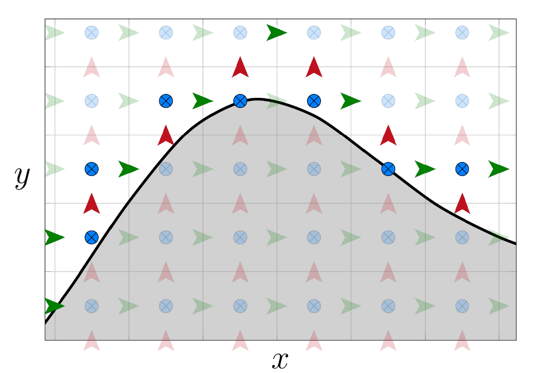
Boundary conditions (BC) are applied on the body or on planar surfaces which must be parallel to the faces of the bounding box. The set of available BC can be extended with little more than defining the new BC itself. More details are provided in the dedicated Section.

Parallelism, domain decomposition and cube pruning

All programs in AMPHIBIOUS run in parallel with MPI; the number of ranks and domain decomposition in every direction can be chosen with maximum flexibility. GPU computing is only available for solver, the only compute-intensive part.

The entire domain is discretized by preproc on a grid made by Nx x Ny x Nz mesh points. It is also decomposed into nDecompCubes = nCubesX x nCubesY x nCubesZ cubic subdomains. Each cube possesses halo points used to exchange data with neighboring cubes. Decomposing the domain into cubes is useful for large cases involving complex geometries; the procedure is inspired by Nakahasi & Kim (2004) and Jansson et al (2019).

A global file general-info.dat and several cube-specific files are written by preproc in the subfolder cubes/. The file general-info.dat contains the value of nTotCubes, the number of non-empty cubes, as well as the list of their IDs. Note that nTotCubes may be less than the total number nDecompCubes, depending on the complexity of geometry and the input parameters nCubesX, nCubesY, nCubesZ. These parameters also determine the MPI preprocessor ranks. Multiple cubes may then be loaded at once by each MPI rank of the solver. Therefore:

• nDecompCubes is the total number of cubes after the initial domain decomposition;
• nTotCubes <= nDecompCubes is the total number of cubes left after the pruning process;
• nCubes <= nTotCubes is the total number of cubes loaded by one MPI rank.

The solver is built such that each MPI rank can be assigned one or more cubes. Therefore, the number of possible MPI ranks ranges from 1 to nTotCubes. When using just one MPI rank, all non-pruned cubes are loaded by the rank; instead, when nTotCubes ranks are used, each rank loads one cube.

The two figures below provide examples where the optimal value for nDecompCubes is chosen by following a different rationale.

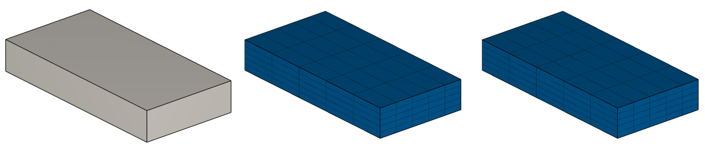
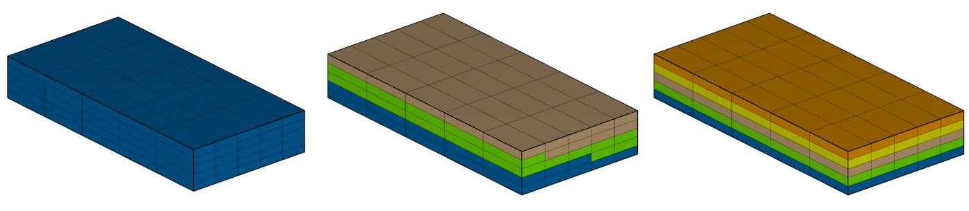
Plane channel flow example. Top: pruning. The bounding box (left) is decomposed in nCubesX=nCubesY=nCubesZ=5 cubes (center); no cubes are pruned (right) as the fluid domain and the bounding box are coincident: nDecompCubes=nTotCubes=125. Bottom: cube-rank assignment, colors identify cubes loaded by each rank. At run time, different MPI ranks can be used, as for example 1 (left), 3 (center) or 5 (right).

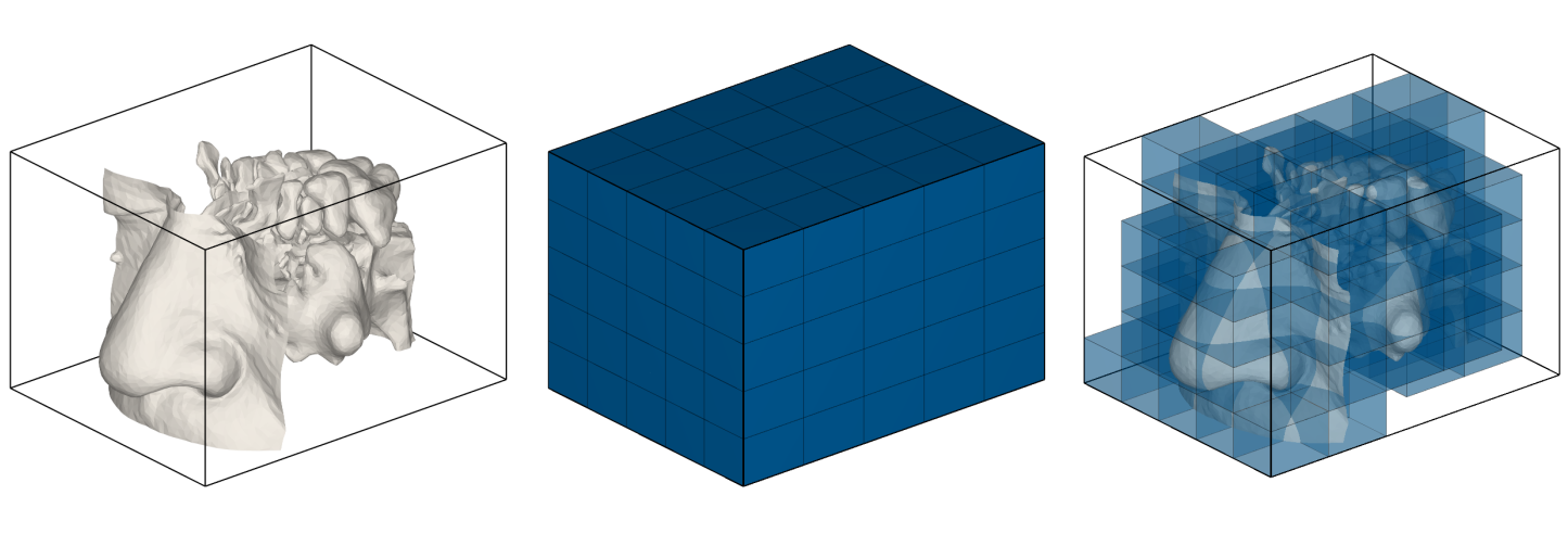
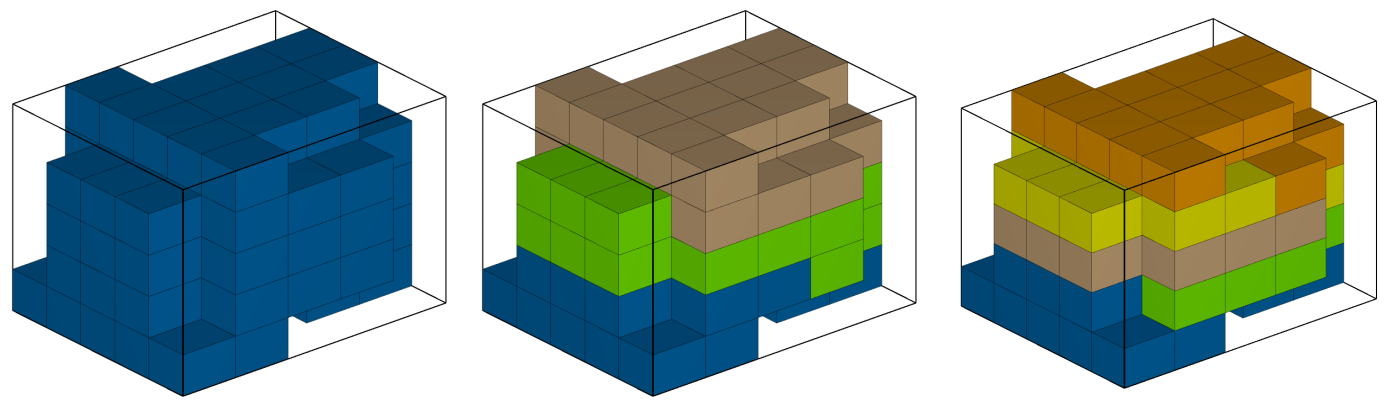
Nose flow example. Top: pruning. The bounding box (left) is decomposed in nCubesX=nCubesY=nCubesZ=5 cubes (center); empty cubes are pruned (right), so that nDecompCubes=125 but nTotCubes=91. Bottom: cube-rank assignment, colors identify cubes loaded by each rank. At run time, different MPI ranks can be used, as for example 1 (left), 3 (center) or 5 (right).

Since each cube may perform up to 26 communications, an excessive number of cubes may lead to a substantial overhead. A large number of cubes is therefore recommended only whenever a load-balancing advantage or significant memory savings are achieved via pruning. Since solver does not alter files written by preproc, experimenting to find the optimal number of ranks for solver is convenient.

Running on GPUs

The compute-intensive solver supports both CPUs and GPUs. GPU programming is implemented using OpenACC directives, which appear in the source code as special comment lines. When running on GPUs, all data structures are copied to GPU at startup, and then permanently reside there. The slow CPU-GPU communications are kept to a minimum: during a time step, such communications only involve single global variables (like e.g. the flow rate). When running on multiple GPUs, GPU-aware MPI communications are used, and explicit CPU-GPU copying is once again avoided. Since the performance degradation caused by multiple MPI ranks working on the same GPU can be substantial (up to 2x slowdown measured), in the multi-GPU case the number of MPI ranks must equal the number of GPUs (a warning is issued otherwise). Load balancing can be performed by properly assigning cubes to MPI ranks, therefore balancing GPU load is not required provided MPI ranks are balanced.

To enable GPU execution, one defines the macro TARGET_IS_GPU in the file headers.cpl. At compile time, the Makefile uses that macro to compile for the intended target.

How to set up a simulation

The simulation process is controlled by a single configuration file, settings.in. Data for one computational experiment are contained within a single directory, the case directory caseDir. The information required for a simulation is:

• a properly filled settings.in, located in <caseDir>;
• the geometrical description of the problem, that can be provided analytically, or through a set of STL files (which, for simple geometries, can be optionally created by hand).

The input file settings.in is organized as a list of independent sections, which can appear in arbitrary sequence. Variables inside a section, instead, must follow the same order as they are READ FROM by the program. An explanatory comment on each line of settings.in helps understanding the meaning of each variable.

The sections are as follows:

• PREPROC:
  sets the variables Nx, Ny, Nz (number of discretization points in each direction) and nCubesX, nCubesY, nCubesZ (number of cubes in each direction);

• NONUNIFORM_GRID:
  whenever the Cartesian grid has non-uniform spacing, sets the law of variation of the grid step, independently for each of the three directions;

• ANALYTIC_GEOMETRY:
  contains the description of a geometry given in analytic form (as in the channel flow example), in terms of box size, number of boundary planes and the corresponding boundary conditions. Alternatively, the section STL_GEOMETRY contains the number and names of the STL files which define the computational domain, each accompanied by the type of boundary condition;

• SOLVER:
  sets fluid properties (e.g. the fluid viscosity nu), as well as parameters for the temporal discretization (e.g. the time step dt), and for the management of the simulation (e.g. the maximum simulation time Tmax); time step can be constant or computed after a CFL condition. The variable nItPressureCorrection sets the number of iterations for the solution of the pressure equation. Physical quantities are expressed in dimensional SI units;

• HT:
  sets properties relative to the heat transfer part of the problem, namely thermalDiffusivity and thermalConductivityRatio. The latter is only used when homogenized BCs are employed, and represent the ratio between the fluid and solid thermal conductivity where the interface problem is solved;

• LES:
  switches between available LES models and allows to tune the models' constant Cm and the Prandtl number prandtlTurb for the turbulence model;

• INPUT_OUTPUT:
  controls whether and how a restart file is saved and used, as well as the creation of a database of flow fields. A set of first and second moments for velocity and pressure can also be computed. Since the full statistics can lead to large file sizes, a subset of statistics can be selected by filling the variable statsNames with the required fields: e.g. statsNames=um,p2 only accumulates the mean of the $u$ velocity component and the variance of pressure fluctuations;

• PROBES:
  controls writing to file time histories of virtual (0d, 1d or 2d) probes placed in the domain; the temporal and spatial frequencies can be regulated with writeProbesEveryTsteps and spaceSampling;

• POSTPROC:
  converts binary data accumulated during the simulation into three-dimensional VTK files for flow field(s) and (velocity and pressure) statistics. The latter can be computed and saved in double or simple precision to save disk space; averaging over homogeneous directions (when present) is also possible to get statistics in an ASCII file;

• a flow-specific section, e.g. CHANNEL_FLOW:
  contains information for the specific flow case; for the channel flow, for example, it contains the enforced value of the flow rate / pressure gradient in two of the three Cartesian directions.

Boundary conditions

The boundary conditions are specified in the *_GEOMETRY section of settings.in. The infrastructure for boundary conditions is such that extensions and refinements are relatively easy. Five BC types are available: no-slip solid wall (w), periodic (p), in-plane moving wall (m), total pressure inlet (i) and total pressure outlet (o). In settings.in, the number of boundaries must be first specified (either as nFaces or nStlFiles for the analytic and STL descriptions, respectively); then, each boundary condition must be prescribed with one line of the type:

type=<bcType> <bcSpec1>=value <bcSpec2>=value ...

where the descriptors <bcType> and <bcSpecs> are described in the following table:

Boundary condition	bcType	bcSpecs	Notes
No-slip solid wall (isothermal, fixed flux or conjugate heat transfer)	w	bcT,bcTn, bcTthickness,bcTbase	Velocity and Dirichlet-type for temperature are managed via the IB coefficients; Neumann-type temperature BC are handled with an optional NeumannData infrastructure
Periodic	p	None	Must be prescribed in pairs
Plane wall with prescribed wall-parallel velocity	m	vel1, vel2, strDistr1, a1, k1, omega1, strDistr2, a2, k2, omega2	None
Total pressure inlet	i	bcP,bcT	None
Total pressure outlet	o	bcP	Homogeneous Neumann is assumed for temperature if needed

With STL geometry, one boundary condition applies to each STL. With analytical geometry, the faces of the bounding box are enumerated starting from $x = x_{min}$, then $x = x_{max}$, and then again for the $y$ and $z$ directions.

• No-slip solid wall This is the standard solid wall, where no-penetration and no-slip boundary conditions are applied via the IB coefficients. The same applies to Dirichlet-type BC for temperature, set by bcT. Constant heat flux is specified through bcTn, whereas bcTthickness and bcTbase specify an approximate solution of the conjugate heat transfer problem. Note that, besides requesting the heat-transfer equation to be solved with the macro USE_HT, whenever the normal derivative of temperature is involved the additional WALLT_IS_NEUMANN must be enabled.

• Periodic Periodic BC must be applied on one (or more) pairs of whole faces of the bounding box. The correct pairing is not explicitly checked.

• Plane wall with prescribed wall-parallel velocity A plane wall can be given a non-zero velocity in the wall-parallel directions. The wall velocity can be spatially non-uniform, and time-dependent as well. The two wall-parallel directions in the Cartesian reference frame are referred to by the indices 1 and 2. The descriptors vel1 and vel2 are constants that can be for example used to prescribe a Couette flow. Time- and space-dependency is limited to sinusoidal variations, with amplitude a1, a2, temporal frequency omega1, omega2 and spatial frequency (wavenumber) k1, k2. The boolean strDistr prescribes whether the sinusoid is streamwise or spanwise. Hence, for a plane wall with normal $y$ with strDistr2=YES, the expression: $$w = vel_2 + a_2 \sin(k_2 x - \omega_2 t)$$ enforces for the spanwise 2 component a travelling wave along the streamwise direction.

• Inlet: total pressure At the inlet boundaries of the computational domain, total pressure is prescribed by assigning a value for the total pressure $p_0$ through the descriptor bcP. Pressure, the velocity component $u_n$ normal to the boundary and the two components $u_{1,p}$ and $u_{2,p}$ parallel to the boundary are prescribed as follows:

  • $u_n$: zero gradient;
  • $u_{1,p} = u_{2,p} = 0$
  • $p = p_0 - \frac{1}{2} V^2$

Temperature, when present, inherits the same BC as velocity. Hence, a constant inlet temperature is specified via bcT

• Outlet: total pressure At the outlet boundaries of the computational domain, total pressure is prescribed by assigning a value for the total pressure $p_0$ through the descriptor bcP. Pressure and velocity components are prescribed in a way that depends on whether, locally, a backflow is present. At points with no backflow, the entire velocity has a zero-gradient condition, and for pressure $p=p_0$. With backflow, pressure is instead set as $p = p_0 - \frac{1}{2} V^2$. Temperature has a zero-gradient condition along the direction normal to the BC plane.

Compilation and dependencies

AMPHIBIOUS is built to be as self-contained as possible, yet some dependencies exist. The current stable version has been tested with the following software:

• the CPL compiler and its (few) dependencies
• a C compiler (current version tested with gcc v.12.2.0 and v.14.2.0) and the nvc compiler for Nvidia GPUs (current version tested with nvc v.23.11 and v.25.1)
• MPI for parallel CPU computing (current version tested with openmpi v.4.1.6 and v.5.0.7 and hpcx-mpi v.2.19); GPU-aware MPI is required for multiGPU computing
• OpenACC >= v.2.6 for parallel (multi)GPU computing

Programs and utilities are compiled with the provided Makefile. The default compiler is gcc for the CPU target and nvc for the GPU target.

Setting the compilation MACROs

The program contains compile-time customization options:

• several macros, which can be optionally set in the file headers.cpl by uncommenting the related #define lines;

• a flow-specific file, placed in the modules-solver/ folder, to be used whenever flow-specific operations in solver are required. To do so, the user must USE it in solver. In the two tutorial examples, the file specifics-channel.cpl manages the screen output at runtime and the forcing term, whereas specifics-nose.cpl only manages the screen output.

The following macros can be set:

Name	Used by	Description
GRID_IS_NONUNIFORM	preproc	Enables non-uniform Cartesian grid in the three directions (default is uniform)
GEOMETRY_IS_ANALYTIC	preproc	Allows preprocessing of analytically-described geometries
WALLT_IS_NEUMANN	preproc	Computes IB coefficients for a Neumann-type temperature BC on the wall
TARGET_IS_GPU	solver	Sets GPU compile target (requires a C compiler supporting OpenACC directives)
STATSIZE_IS_DOUBLE	solver postproc	Computes statistics in double precision (default is single precision)
USE_LES	solver postproc	Toggles use of LES model, either at run time or to compute the field of $\nu_t$ in post-processing
USE_HT	solver postproc	Switches on the equation for the passive scalar (heat transfer)

Flow-specific files can be used by solver to customize its behavior. In the tutorials, the file specifics-channel.cpl manages the runtime screen output and the forcing term, and includes initial conditions for laminar Poiseuille and Couette flows, as well as a laminar Stokes layer profile on one wall, with optional deterministic and/or random perturbations. In specifics-nose.cpl, instead, only the screen output is specified. When needed, flow-specific input can be assigned in a dedicated section in the settings.in file. Any ad hoc routine defined in the flow-specific files is INLINEd. By doing so, solver variables can be accessed even when still undefined (of course, they must be defined when the function is called). The CPL deferred assignment operator == must be used. An example can be found in specifics-channel.cpl.

The case directory and its structure

preproc, solver and postproc all read and write files to/from the case folder <caseDir>, where they are organized in subfolders. Subfolders have constant names. The file names, instead, are as follows:

• a fixed part, which informs of the content of the file (e.g. restart);
• a variable part, which is unique for each cube, based on cube ID and the total number of cubes nDecompCubes;
• the extension of the file (e.g. .vtk or .bin).

For example, by executing the program serially, the restart file is called restart.1of1.bin as only one cube is generated.

After the execution of postproc, the case directory is fully populated and presents the following structure:

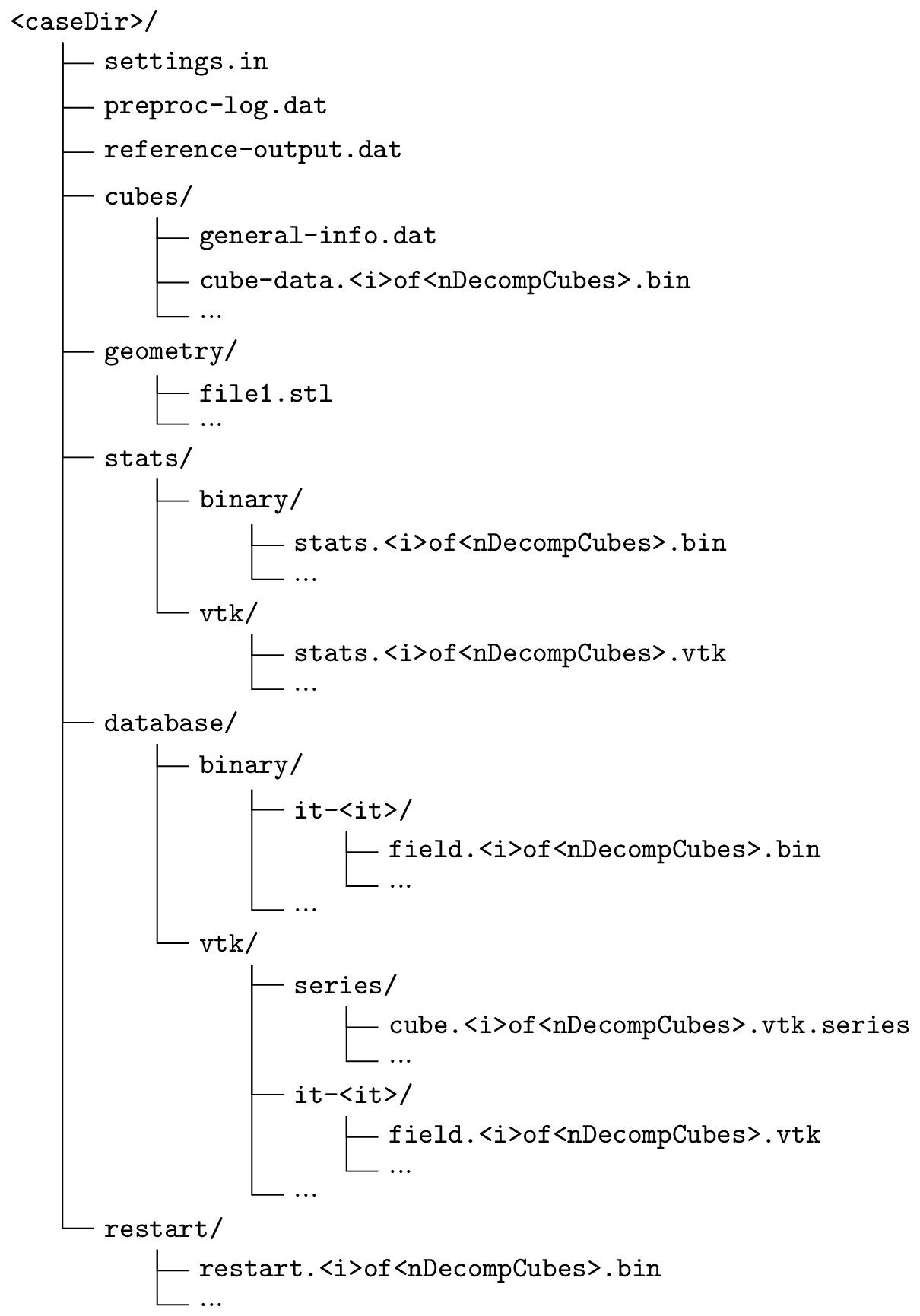
Structure of a case folder (the file reference-output.dat is only present in the tutorials).

The cube-specific files are made by two parts:

• an ASCII header, whose length of 8kB is set in headers.cpl, which contains cube data and metadata, e.g. cube connectivity for the cube-data files, or the snapshot timestamp in the restart files
• a binary chunk, which contains the saved data (e.g. IB coefficients, accumulated statistics, restart field, snapshots).

Binary data are written on file in the way they are organized in memory at run time, i.e. with SoA ordering (Structure of Arrays) in row-major order (as in C language: arrays are indexed with the most rapidly changing index last). The data structure is written to disk without discriminating between internal or external points. Not all data structures share the same size: IB coefficients, restart fields and snapshots data structures are defined also in the halo points of the cube, while statistics are not.

Performance

Performance analysis is still preliminary, and certain parts of the code do require substantial optimization. Nevertheless, the starting point in terms of raw computational performance is encouraging. The figure below illustrates the measured time, normalized for point and time (sub)step, for CPU and GPU execution, on a problems sized 1024³ (strong scaling). The test hardware is the Leonardo Booster partition at CINECA. Each of the 3456 nodes has a single socket Intel Xeon Platinum 8358 with 32 cores, and four NVIDIA A100 GPUs with 64 GB RAM. The node has 512 GB DDR4 RAM; inter-node communications are serviced through NVIDIA Mellanox Infiniband with 200 Gbps and DragonFly+ topology. The GPUs in a node are interconnected through NVLink 3.0 for peer-to-peer memory transfers.

Strong scaling on CPUs and GPUs (preliminary data).

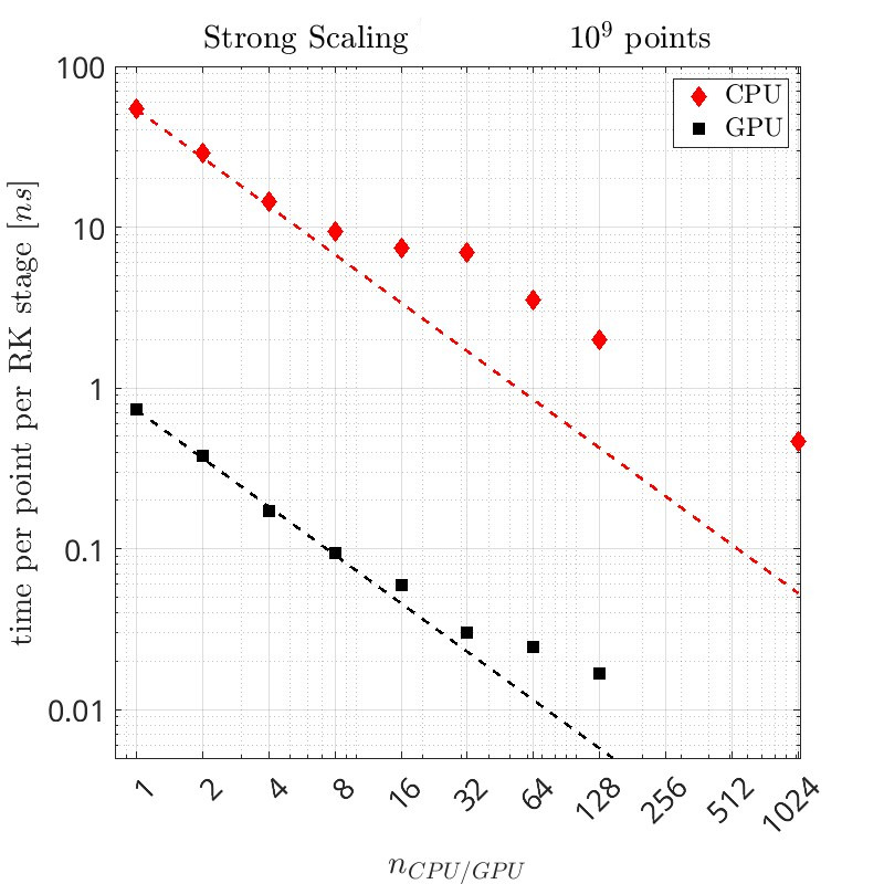
The CPU execution has a scalar speed of 55 x 10^-9 seconds per point/step on one core; efficiency is gradually affected until the cores of the first node get fully used. After that, linear scaling is observed up to the maximum tested number of 1024 cores. The GPU execution has a single-GPU speed of 7.5 10^-10 seconds per point/step: a case of size 1024³ advances by one time step in 0.75 seconds. The multi-GPU scaling is approximately linear up to 32 GPUs, and then starts to drift gradually. Note how the memory efficiency allows us to run a relatively large case with over a billion points on a single core. In fact AMPHIBIOUS needs about 120 bytes per (internal) point, plus 4/8 additional bytes for each quantity for which statistics are accumulated.

Running a simulation

In the Tutorials section, simple cases are presented with comments and a step-by-step guide. Instructional videos are also available.

The typical workflow involves the sequential run of preproc, solver and possibly postproc, once the simulation is set up by preparing the settings.in file (and by providing STL files, when required).

Data are read from/written to files residing in a single user-defined directory, the case directory caseDir. Each program is executed as:

mpirun -n <N> <program> <caseDir>

where <program> is ./preproc, ./solver or ./postproc, N is the number of MPI ranks, and <caseDir> is where the settings.in file is located.

The execution model of AMPHIBIOUS assumes that source, macros and the settings file settings.in are changed wisely amid the execution of a case, i.e. between two steps of the execution pipeline preproc-solver-postproc.